Tutorial 1: running floria and visualizing its outputs
This minimal tutorial goes over floria’s inputs and outputs by running floria on toy data. We will show how to visualize and interpret floria’s outputs.
Prerequisites and running floria
We will assume that you’ve installed floria and took a look through Introduction. See the Quick start page if you have not installed floria. Once floria is installed, run the following commands.
# clone the repository if you have not done so
git clone https://github.com/bluenote-1577/floria
cd floria

# assuming you've installed floria
floria -b tests/test_long.bam -v tests/test.vcf -r tests/MN-03.fa -o example_output
ls example_output
For visualization, you will need:
IGV installed.
matplotlib, numpy, python3 installed for vartig visualization.
samtools in PATH and pysam installed for IGV visualization.
Running pip install pysam numpy matplotlib should do the trick if you don’t have these dependencies installed. samtools can easily be installed via conda or built manually, but make sure it is in PATH if you want to do IGV visualization.
Inputs
The provided files represent a mixture of synthetic Klebsiella Pneumoniae reads for three different strains.
test_long.bam represent synthetic nanopore reads from three different strains at 70x, 30x, and 10x coverage. We then mapped these reads to the MN-03.fa reference genome to generate the bam file. We only retained reads between positions 1-120,000 for this example.
test.vcf was obtained by calling SNPs on test_long.bam. We used longshot, a long-read SNP caller to call these SNPs.
MN-03.fa is the contig we mapped onto. This is an arbitrary Klebsiella Pneumoniae strain.
Output log
Depending on your version of floria, you should see something like the following after running the command.
2023-06-12T23:33:40.561Z INFO  [floria::file_reader] 33,50,66 non-hard clipped read length percentiles: 9943, 13066, 16494. If -l is not set, estimated -l is set to 16494.
2023-06-12T23:33:40.561Z INFO  [floria::file_reader] If -e is not set, estimated -e is set to 0.04081632653061224.
2023-06-12T23:33:40.563Z INFO  [floria] Preprocessing VCF/Reference
2023-06-12T23:33:40.568Z INFO  [floria] Finished preprocessing in 5.20466ms
2023-06-12T23:33:40.568Z INFO  [floria] Reading and realigning inputs for contig NZ_CP081897.1 (BAM/VCF).
2023-06-12T23:33:40.664Z INFO  [floria] Contig NZ_CP081897.1 has 954 SNPs
2023-06-12T23:33:40.664Z INFO  [floria] Reading inputs, realigning time taken 96.312178ms
2023-06-12T23:33:40.664Z INFO  [floria] Local phasing with 20 threads...
2023-06-12T23:33:41.041Z INFO  [floria] Phasing time taken 376.723842ms
2023-06-12T23:33:41.041Z INFO  [floria] Solving flow problem...
2023-06-12T23:33:41.041Z INFO  [floria] Flow solved in time 339.672µs
2023-06-12T23:33:41.084Z INFO  [floria::file_writer] Final SNP error rate for all haplogroups is 0.05546256145299258
2023-06-12T23:33:41.085Z INFO  [floria] Total time taken is 522.39064ms
The “Total time …” line indicates floria has exited successfully. A few lines that may be of interest:
The first line indicates what the
-lparameter, the block length.The second line indicates how we estimate the
-eparameter, the baseline error rate. The user can also supply this.The line “Final SNP error rate …” describes the fraction of alleles that are discordant in your final outputs.
For understanding the -l and -e parameters, see Guide: optimizing parameters for phasing.
floria’s main outputs
The output structure is outlined in Outputs in detail, and a more detailed description of each output file is also in the link. Let’s go over the important files.
contig_ploidy_info.tsv
 cat example_output/contig_ploidy_info.tsv
 ------------------------------------------
contig       average_straincount     whole_contig_multiplicity       approximate_coverage_ignoring_indels    total_vartig_bases_covered      average_straincount_min15hapq   average_straincount_min30hapq   average_straincount_min45hapq   avg_err
NZ_CP081897.1        3.000   0.068   79.601  354838  2.984   2.984   1.000   0.0555
This file gives information about how many strains appear to be present in our sample. For each contig, a line will be present in this file. We only have one contig, so we only get one (non-header) line.
The most important columns are usually columns 2-4.
average_global_straincountsuggests how many strains there are. In our case, it looks like there are exactly 3 strains present, which is correct.whole_contig_multiplicityis simply the sum of vartig lengths divided by contig length. Here we have around 360,000 total bases covered by vartigs (column 6), which is good (3 strains x 120,000 bases). The complete genome is about 5 Mb, hence 0.068 is the result – implying only part of the genome is phased.approximate_coverage_ignoring_indelsgives an estimate of the coverage. The true coverage is 110x here, but we only get ~80x coverage. This is because our simulated nanopore reads had a lot of indels, which causes reads skip over alleles, lowering our estimated coverage.
See Guide: understanding output phasings and their pitfalls for more information on interpreting this file.
NZ_CP081897.1.haplosets
For the rest of the files, they are stored in example_output/NZ_CP081897.1. floria outputs results for each contig in the bam file. Because we only have one contig, there is only one output folder. Let’s start with the NZ_CP081897.1.haplosets file.
The *.haplosets file is present for every contig phased. This describes the strain-level read clusters output by floria.
> head example_output/NZ_CP081897.1/NZ_CP081897.1.haplosets
------------------------------------------------------------
>HAP0.example_output/NZ_CP081897.1  CONTIG:NZ_CP081897.1    SNPRANGE:1-15   BASERANGE:771-3416      COV:2.429       ERR:0.088       HAPQ:0  REL_ERR:1.591
nc1_20364   2       12
nc1_5047    3       15
nc1_13853   3       14
>HAP1.example_output/NZ_CP081897.1  CONTIG:NZ_CP081897.1    SNPRANGE:1-954  BASERANGE:771-119079    COV:49.374      ERR:0.075       HAPQ:47 REL_ERR:1.346
nc1_929     1       110
nc1_30767   1       59
nc1_35492   1       35
nc1_16553   1       26
nc1_35227   2       71
...
The first line with the > gives information about the haploset. Again, all of the flags are described in Outputs, but let’s go over the important ones.
The first haploset is called
HAP0, and it covers the SNPs through [1,15] (inclusive interval).The bases it covers are [771,3416], which corresponds to SNPs [1,15].
The
COVis 2.429, so it is does not have high coverage.The
HAPQis 0.
The rest of the lines indicate which reads are contained in the haploset, and what SNP positions each read covers. The first read covers [2,12], for example.
Interpreting the haploset information
It looks like the first haploset is a small set containing only 3 long-reads, and not covering much of the genome. The low HAPQ is indicative that this phasing may be spurious. HAPQ does not indicate if the phasing is good, just whether or not it may be spurious.
By “spurious”, we mean “Does this phasing really represent the existence of a strain?”
By “good” we mean, “Are there errors in this phasing? e.g. are there switch errors?”
Note
HAPQ can be interpreted like MAPQ for reads. E.g. High MAPQ does not indicate high sequence identity, but it indicates a good confident mapping position.
So our HAPQ is 0; is this fair? Well, it turns out our reads have prefixes that indicate what strain they came from (because we simulated our reads). As can be seen below:
> cat example_output/NZ_CP081897.1/NZ_CP081897.1.haplosets
------------------------------------------------------------
>HAP0.example_output/NZ_CP081897.1  CONTIG:NZ_CP081897.1    SNPRANGE:1-15   BASERANGE:771-3416      COV:2.429       ERR:0.088       HAPQ:0  REL_ERR:1.591
nc1_20364   2       12
nc1_5047    3       15
nc1_13853   3       14
>HAP1.example_output/NZ_CP081897.1  CONTIG:NZ_CP081897.1    SNPRANGE:1-954  BASERANGE:771-119079    COV:49.374      ERR:0.075       HAPQ:47 REL_ERR:1.346
nc1_929     1       110
nc1_30767   1       59
nc1_35492   1       35
nc1_16553   1       26
nc1_35227   2       71
...
>HAP2.example_output/NZ_CP081897.1      CONTIG:NZ_CP081897.1    SNPRANGE:1-954  BASERANGE:771-119079    COV:23.742      ERR:0.019       HAPQ:38 REL_ERR:0.349
mn1_15098       1       16
mn1_2680        3       75
mn1_15393       3       48
mn1_14763       3       39
mn1_8191        3       26
...
>HAP4.example_output/NZ_CP081897.1      CONTIG:NZ_CP081897.1    SNPRANGE:16-954 BASERANGE:3502-119079   COV:6.549       ERR:0.041       HAPQ:36 REL_ERR:0.744
pa1_5458        21      73
nc1_10985       22      23
nc1_35501       23      23
pa1_2856        24      111
pa1_272 33      202
pa1_3056        33      46
pa1_344 46      56
pa1_983 47      131
pa1_1945        53      251
pa1_127 53      75
pa1_2033        59      136
pa1_4379        67      73
...
It turns out that HAP0 is a false haplotype after looking at this file in more detail.
HAP1is a much longer version ofHAP0, capturing thenc1strain.HAP2captures themn1strain.HAP4(notice the skip; haplotype numbering can skip) captures thepa1strain, although some shortnc1reads are mixed in.
so it’s good we assumed 0 to the HAPQ.
NZ_CP081897.1.vartigs
We may care about the sequence of alleles that are present on the haplotype represented by the haploset. We will call these vartigs, which are analogous to contigs but on the variant (SNP) level, not on the base level. This is found in the example_output/NZ_CP081897.1/NZ_CP081897.1.vartigs file.
cat example_output/NZ_CP081897.1/NZ_CP081897.1.vartigs
------------------------------------------------------
>HAP0.example_output/NZ_CP081897.1  CONTIG:NZ_CP081897.1    SNPRANGE:1-15   BASERANGE:771-3416      COV:2.429       ERR:0.088       HAPQ:0  REL_ERR:1.591
?11111111111111
>HAP1.example_output/NZ_CP081897.1  CONTIG:NZ_CP081897.1    SNPRANGE:1-954  BASERANGE:771-119079    COV:49.374      ERR:0.075       HAPQ:47 REL_ERR:1.346
11111111111111111111111111111111111111...
>HAP2.example_output/NZ_CP081897.1  CONTIG:NZ_CP081897.1    SNPRANGE:1-954  BASERANGE:771-119079    COV:23.742      ERR:0.019       HAPQ:38 REL_ERR:0.349
00000000000000000000000000000000000000...
>HAP4.example_output/NZ_CP081897.1  CONTIG:NZ_CP081897.1    SNPRANGE:16-954 BASERANGE:3502-119079   COV:6.549       ERR:0.041       HAPQ:36 REL_ERR:0.744
?????011000010101010101011110010011111...
The header info in the vartig file is in the same format. However, instead of representing groups of reads, the vartig gives the sequence of SNPs in the haplosets.
The allele
0represents the reference allele.The allele
1represents the first alternate allele.2would represent the second, and so forth.The allele
?represents no reads in that haploset cover the allele, so it is unknown.
We truncated the vartigs in the above output, but HAP1 has almost all alleles 1 in the range [1,954], whereas HAP2 has 0 on almost all alleles. HAP4 is a mix of 0 and 1. This makes sense; it turns out the reads in HAP2 are simulated from the reference genome MN-03.fa, so it makes sense that HAP2 is almost all reference (any 1 alleles for HAP2 would be errors).
Note
Notice that the ERR for the vartigs increases as the number of alternate alleles increases. This is called reference bias; SNP calls are biased towards the reference, so true alternate alleles are called less often.
reads_without_snps.tsv
This file captures any reads that do not have SNPs present (e.g. reads that are too short) or are placed in regions without any SNPs. In our example, there are SNPs throughout the genome, so this file is empty.
vartig_info.txt
For more information about the haplosets/vartigs, look at the files in example_output/NZ_CP081897.1/vartig_info/*. These files give more information about how confident we are in each allele call for each vartig. See Outputs.
Outputting reads
By default, floria only outputs read ids for the phased haplosets. If you want the base-level reads, use the --output-reads option. If you look at example_output/NZ_CP081897.1/long_reads, you’ll see the folder is empty, but we can rerun floria:
# need to specify --overwrite and --output-reads
floria --overwrite --output-reads -b tests/test_long.bam -v tests/test.vcf -r tests/MN-03.fa -o example_output
and now the reads appear like example_output/NZ_CP081897.1/long_reads/2_part.txt. These are the reads corresponding to HAP2. Importantly, these reads are trimmed against the haploset and may not represent the original reads. See Read output for more information.
Visualizing vartigs/haplosets
To visualize your vartigs, we provide a script called visualize_vartigs.py in the following repository scripts folder of the floria github repository. You will need numpy and matplotlib installed. Simply run:
python scripts/visualize_vartigs.py example_output/NZ_CP081897.1/NZ_CP081897.1.vartigs
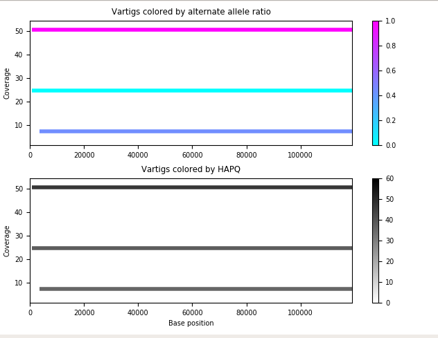
You should see the above figure. In a nutshell:
Each bar represents a vartig with HAPQ > 0.
The y-axis represents the COV for the vartig, and the x-axis represents the BASERANGE of the vartig.
The upper plot colors the vartig by alternate allele fraction. That is, what percentage of the vartig contains non
0alleles.The lower plot colors the vartig by HAPQ.
We have three true strains here, which are well represented by this plot.
We’ve found the above visualization to be very useful in practice for confirming that a phasing is reasonable. If you have a consistent coverage level and alternate allele fraction, you can be confident that your phasing is reasonable. For example, the second picture is a phasing for a real nanopore community with a slightly different colormap:
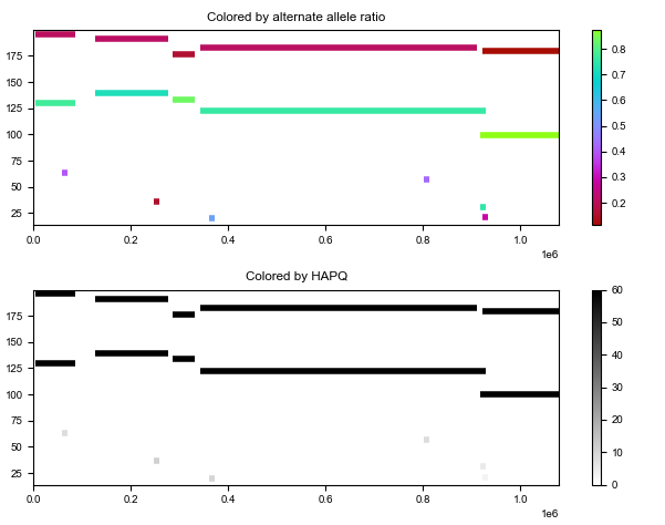
Notice that alternate allele fraction is relatively constant and that coverage is consistent, even across broken vartigs.
Visualizing haplosets via IGV
To visualize the actual reads in the haplosets instead of just the vartig, we provide the script floria/scripts/haplotag_dir.py. This script outputs a bam file with haplotagging information, a field in the BAM record that indicates which phasing a read comes from.
python scripts/haplotag_output_dir.py -d example_output/ -b tests/test_long.bam -o haplotagged_example
ls haplotagged_example.bam haplotagged_example.bam.bai
For more in-depth information on how to use the IGV, see any tutorial out there. Briefly, once you have the IGV open, simply
Load the
haplotagged_example.bamfile in the upper left “File -> Load from file” menu.Load
MN-03.faas the reference in the “Genomes -> Load genome from file” menu.Right click the left panel, click “Group alignments by” and then “phase”.
Right click the left panel, and choose “squished”.
Zoom into your area of interest.
You should then see the following picture.
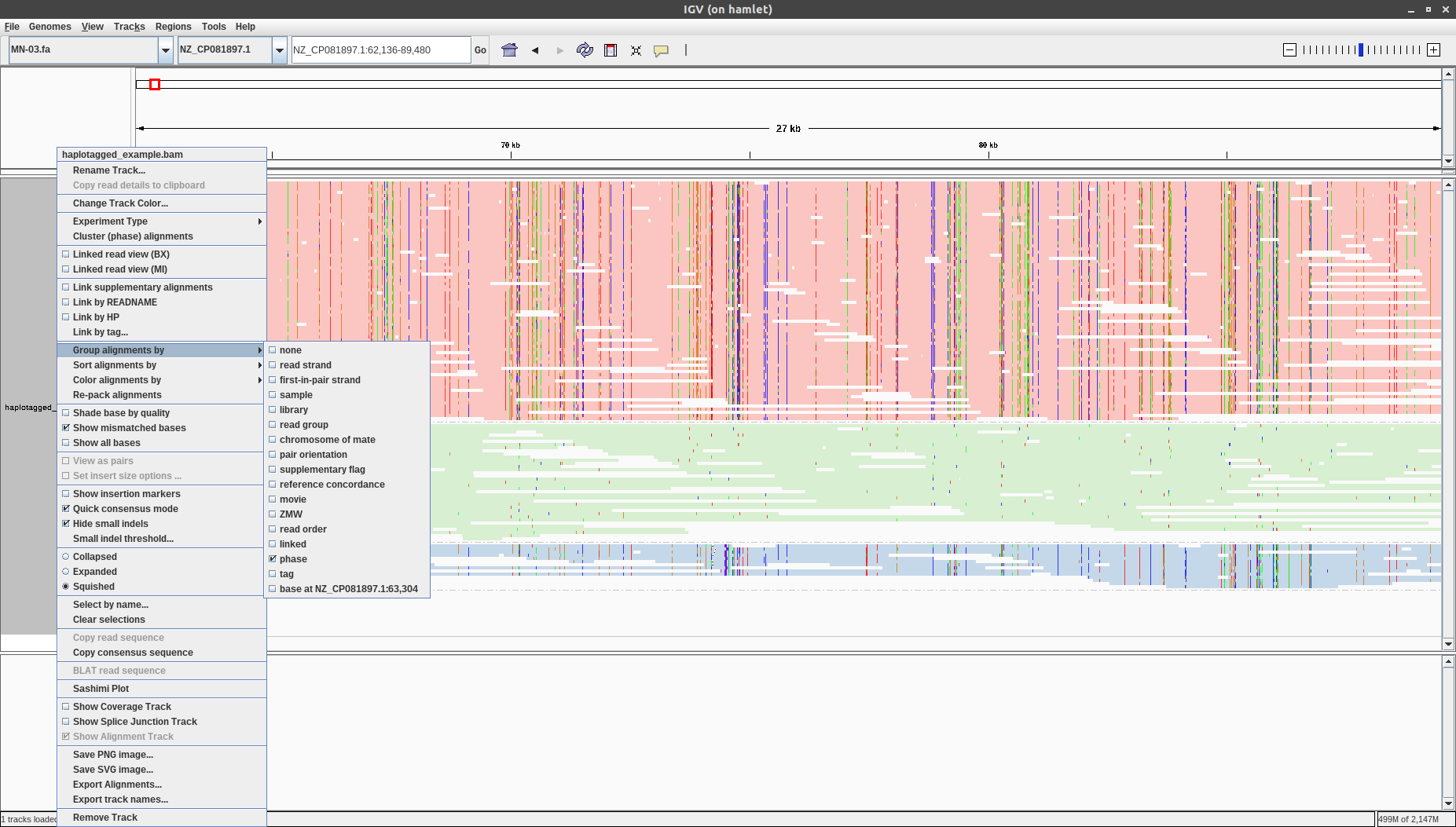
Notice the HAP number are shown on the left hand side. HAP0 is not output because we do not output haplosets with HAPQ = 0.
Summary: floria is not perfect, and we recommend visualizing in IGV manually if you can. In practice, this is a very useful way of manually confirming that floria’s haplosets are reasonable. It is a bit more inconvenient than the visualize_vartigs.py script, but it is more comprehensive and helpful when visualize_vartigs.py’s output is messy.
Conclusion
We’ve shown how to run floria on a toy synthetic 3 strain mock community. floria offers sane defaults, a simple command line for phasing, and two very useful tools for visualizing results.